の続き
lmfitは、複数の2次元正規分布でもフィッティングができる
gauss = lmfit.models.Gaussian2dModel(prefix="g1")
params = gauss.make_params()
model = gauss

gauss = lmfit.models.Gaussian2dModel(prefix="g2")
params.update(gauss.make_params())
model = model+gauss
パラメータに拘束条件をつけることもできる。
これは、g2sigmax = g1sigmax 、 g2sigmay = g1sigmay の意味。
params["g2sigmax"].set(expr="g1sigmax")
params["g2sigmay"].set(expr="g1sigmay")
コード全体
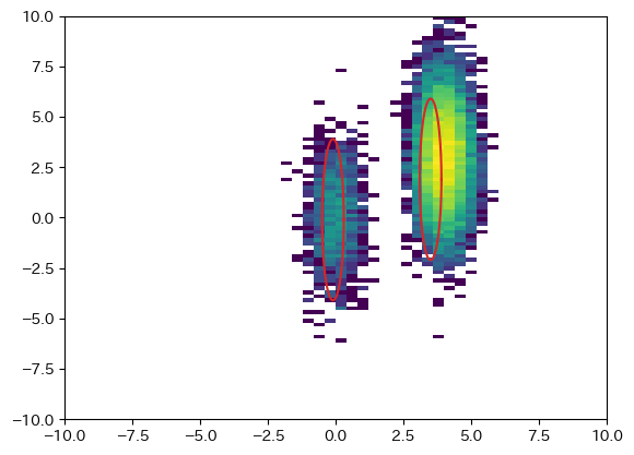
import numpy as np
import lmfit
from lmfit.lineshapes import gaussian2d, lorentzian

np.random.seed(0)
x0 = np.random.randn(10000)*0.5 + 4 #標準偏差0.5, 平均4の正規分布
y0 = np.random.randn(10000)*2   + 3 #標準偏差2.0, 平均3の正規分布
x1 = np.random.randn(1000)*0.5 + 0 #標準偏差0.5, 平均0の正規分布
y1 = np.random.randn(1000)*2   + 0 #標準偏差2.0, 平均0の正規分布

x=np.concatenate((x0,x1))
y=np.concatenate((y0,y1))

xrange=[-10,10]
yrange=[-10,10]
bins=[50,100]

hist, edgesx, edgesy = np.histogram2d(x,y,bins=bins,range=[xrange,yrange])
arr_x = []
arr_y = []
arr_z = []
arr_zerror = []
for ix,vx in enumerate((edgesx[:-1]+edgesx[1:])*0.5):
    for iy,vy in enumerate((edgesy[:-1]+edgesy[1:])*0.5):
        if hist[ix,iy]==0:continue
        arr_x.append(vx)
        arr_y.append(vy)
        arr_z.append(hist[ix,iy])
        arr_zerror.append(hist[ix,iy]**0.5)

arr_zerror = np.array(arr_zerror)

gauss = lmfit.models.Gaussian2dModel(prefix="g1")
params = gauss.make_params()
model = gauss

gauss = lmfit.models.Gaussian2dModel(prefix="g2")
params.update(gauss.make_params())
model = model+gauss

params["g1centerx"].set(value=3.5,max=5,min=2)
params["g1centery"].set(value=1.9,max=3,min=1)
params["g1sigmax"].set(value=0.2)
params["g1sigmay"].set(value=2)

params["g2centerx"].set(value=-0.1,max=0.5,min=-0.5)
params["g2centery"].set(value=-0.1,max=0.5,min=-0.5)
params["g2sigmax"].set(expr="g1sigmax")
params["g2sigmay"].set(expr="g1sigmay")

#楕円の点列作成
def get_ellipse_xy(centerx, sigmax, centery, sigmay):
    t = np.linspace(0, 2*np.pi, 100)
    x = sigmax*2 * np.cos(t)
    y = sigmay*2 * np.sin(t)
    return x+centerx, y+centery

import matplotlib.pyplot as plt
import matplotlib

#初期値のグラフを描く
plt.hist2d(x,y,bins=bins,range=[xrange,yrange], norm=matplotlib.colors.LogNorm())
for prefix in ["g1","g2"]:
    plt.plot(*get_ellipse_xy(*[params[prefix+mem].value for mem in ['centerx','sigmax','centery','sigmay']]),color="tab:red")
plt.show()

#フィッティング
result = model.fit(arr_z, x=arr_x, y=arr_y, params=params, weights=1.0/arr_zerror, scale_covar=False)
lmfit.report_fit(result)

#フィット後のグラフを描く
plt.hist2d(x,y,bins=bins,range=[xrange,yrange], norm=matplotlib.colors.LogNorm())
for prefix in ["g1","g2"]:
    plt.plot(*get_ellipse_xy(*[result.result.params[prefix+mem].value for mem in ['centerx','sigmax','centery','sigmay']]),color="tab:red")
plt.show()
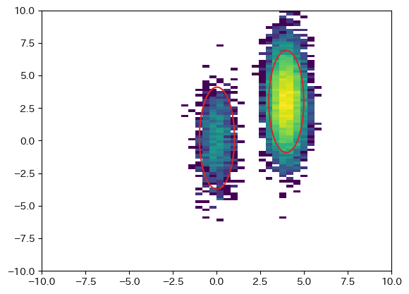
結果
図中の楕円は2σのライン
[[Fit Statistics]]
    # fitting method   = leastsq
    # function evals   = 161
    # data points      = 679
    # variables        = 8
    chi-square         = 568.042626
    reduced chi-square = 0.84656129
    Akaike info crit   = -105.150348
    Bayesian info crit = -68.9853788
[[Variables]]
    g1amplitude:  774.765317 +/- 7.90402876 (1.02%) (init = 1)
    g1centerx:    3.98680648 +/- 0.00516811 (0.13%) (init = 3.5)
    g1centery:    3.00000000 +/- 4.4017e-05 (0.00%) (init = 1.9)
    g1sigmax:     0.50043538 +/- 0.00374820 (0.75%) (init = 0.2)
    g1sigmay:     1.95719965 +/- 0.01511816 (0.77%) (init = 2)
    g1fwhmx:      1.17843524 +/- 0.00882635 (0.75%) == '2.3548200*g1sigmax'
    g1fwhmy:      4.60885287 +/- 0.03560055 (0.77%) == '2.3548200*g1sigmay'
    g1height:     1242.53007 +/- 18.3067883 (1.47%) == '1.5707963*g1amplitude/(max(1e-15, g1sigmax)*max(1e-15, g1sigmay))'
    g2amplitude:  69.4744491 +/- 2.44157021 (3.51%) (init = 1)
    g2centerx:    0.02245085 +/- 0.01950439 (86.88%) (init = -0.1)
    g2centery:    0.19129074 +/- 0.07640330 (39.94%) (init = -0.1)
    g2sigmax:     0.50043538 +/- 0.00374820 (0.75%) == 'g1sigmax'
    g2sigmay:     1.95719965 +/- 0.01511816 (0.77%) == 'g1sigmay'
    g2fwhmx:      1.17843524 +/- 0.00000000 (0.00%) == '2.3548200*g2sigmax'
    g2fwhmy:      4.60885287 +/- 0.00000000 (0.00%) == '2.3548200*g2sigmay'
    g2height:     111.419665 +/- 3.91566886 (3.51%) == '1.5707963*g2amplitude/(max(1e-15, g2sigmax)*max(1e-15, g2sigmay))'
確かに、g1sigmaxとg2sigmax、g1sigmaxとg2sigmayのフィット結果は同じになっている。