線形補間
# サンプルデータを取得
import urllib.request
with urllib.request.urlopen("https://gitlab.com/gifuescan/atima_rangeenergy/-/raw/1e7c7d1432c302d0705a5ea9fe40d696ec468e54/splines_emul_1.41/BeamZ1_TargetZ6.txt") as web_file:
    data = web_file.read()
    with open("BeamZ1_TargetZ6.txt", mode='wb') as local_file:
        local_file.write(data)

import numpy as np
data = np.loadtxt("BeamZ1_TargetZ6.txt")
内挿は簡単でデータ点を詰めて関数を取得する。kindは‘linear’, ‘nearest’などが使えるが、今回は'cubic'にした。
# 内挿する関数
from scipy import interpolate
f = interpolate.interp1d(data.T[0], data.T[1], kind='cubic')
print(f(0.5))
以下、内挿の関数やデータは全く使わない。 積分(Cumulatively integrate)も同じくデータ点を詰めて初期値を与えるだけである。dEdx[MeV cm2/g]の逆数をエネルギー[MeV]で積分するとRange[g/cm2]が得られるので、
#dE/dxとEnergyからRangeを数値計算の積分で求める
from scipy import integrate
Energy = data.T[0]
dEdx = data.T[1]/1000.0
Range = integrate.cumtrapz(1.0/dEdx, Energy, initial=0)
描画をしておく
#描画
import matplotlib.pyplot as plt
plt.plot(Energy, data.T[2], 'r.', label="Original")
plt.plot(Energy, Range, 'b-', label="Integral")
plt.xscale("log")
plt.xlabel("Energy [MeV]")
plt.yscale("log")
plt.ylabel(r"Range [mg/cm2]")
plt.legend()
plt.show()

import matplotlib.pyplot as plt
plt.plot(Energy[1:], (Range[1:]/data.T[2][1:]-1)*100, 'b-')
plt.xscale("log")
plt.xlabel("Energy [MeV]")
plt.ylim(-0.1,0.1)
plt.ylabel("Difference [%]")
plt.grid(True)
plt.show()
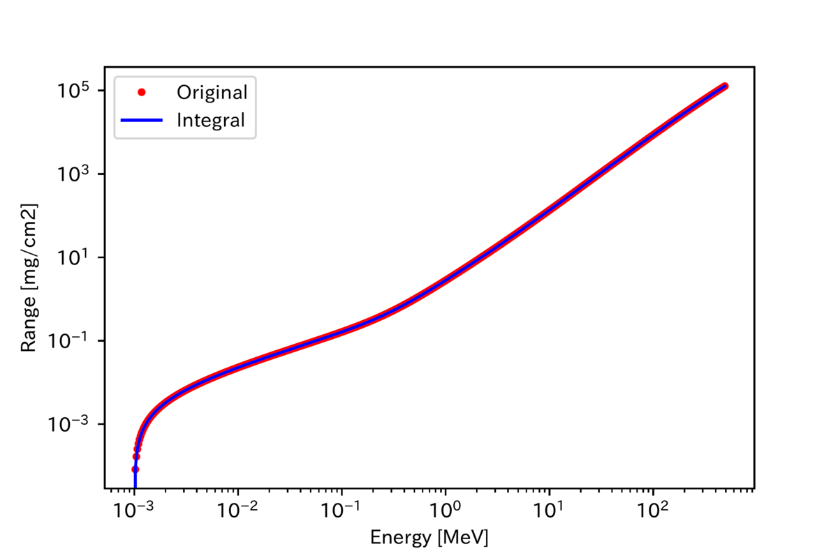
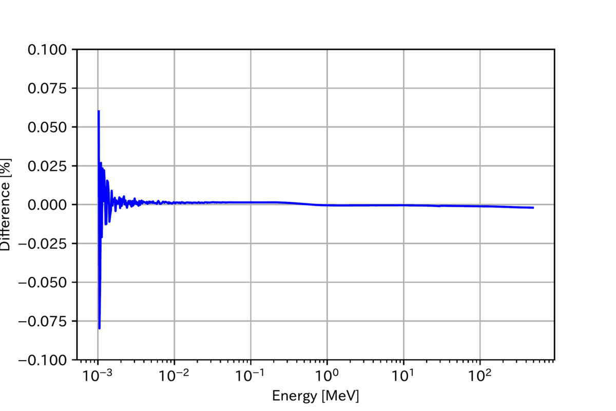
多少の誤差はあるが概ね積分がうまくいっているようだ。